About LLM part 1

26 Jun, 2025 • 6 min read

Root Mean Square Layer Normalization

Layer normalization (LayerNorm) has been successfully applied to various deep neural networks to help stabilize training and boost model convergence because of its capability in handling re-centering and re-scaling of both inputs and weight matrix. However, the computational overhead introduced by LayerNorm makes these improvements expensive and significantly slows the underlying network. LayerNorm was widely accepted because it’s simplicity and no dependence among training cases and it also handle variable length inputs unlike BatchNorm. Unfortunately, the incorporation of LayerNorm raises computational overhead. Although this is negligible to small and shallow neural models with few normalization layers, this problem becomes severe when underlying networks grow larger and deeper. As a result, the efficiency gain from faster and more stable training (in terms of number of training steps) is counter-balanced by an increased computational cost per training step, which diminishes the net efficiency. One major feature of LayerNorm that is widely regarded as contributions to the stabilization is its recentering invariance property.

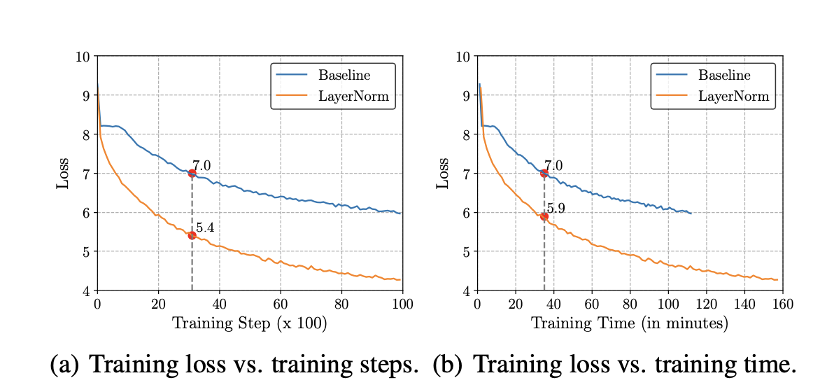
RMSNorm which only focuses on re-scaling invariance and regularizes the summed inputs simply according to the root mean square (RMS) statistic RMS Norm Equation $$ \mathrm{RMS} = \sqrt{\frac{1}{n} \sum_{i=1}^{n} x_i^2} $$

A well-known explanation of the success of LayerNorm is its re-centering and re-scaling invariance property. The former enables the model to be insensitive to shift noises on both inputs and weights, and the latter keeps the output representations intact when both inputs and weights are randomly scaled

Positional Encoding

Desirable Properties

Each position needs a unique encoding that remains consistent regardless of sequence length
The relationship between positions should be mathematically simple. If we know the encoding for position p, it should be straightforward to compute the encoding for position p+k, making it easier for the model to learn positional patterns.
It would be ideal if our positional encodings could be drawn from a deterministic process. This should allow the model to learn the mechanism behind our encoding scheme efficiently.

Drawbacks of absolute positonal encoding

Don’t capture relative position between tokens
While absolute positional encoding captures the positional information for a word, it does not capture the positional information for the entire sentence

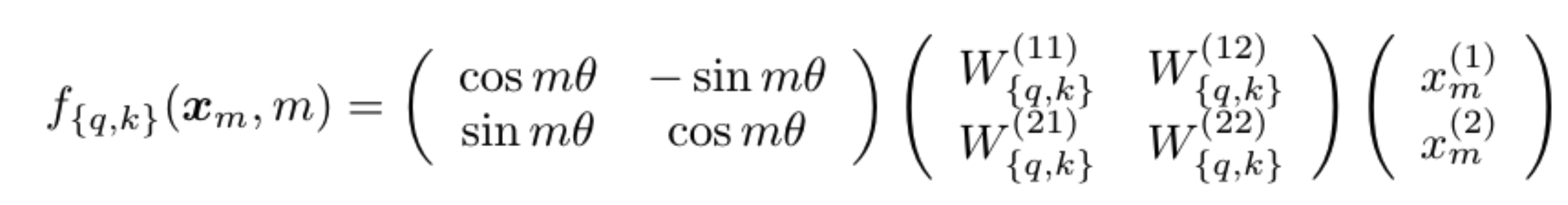
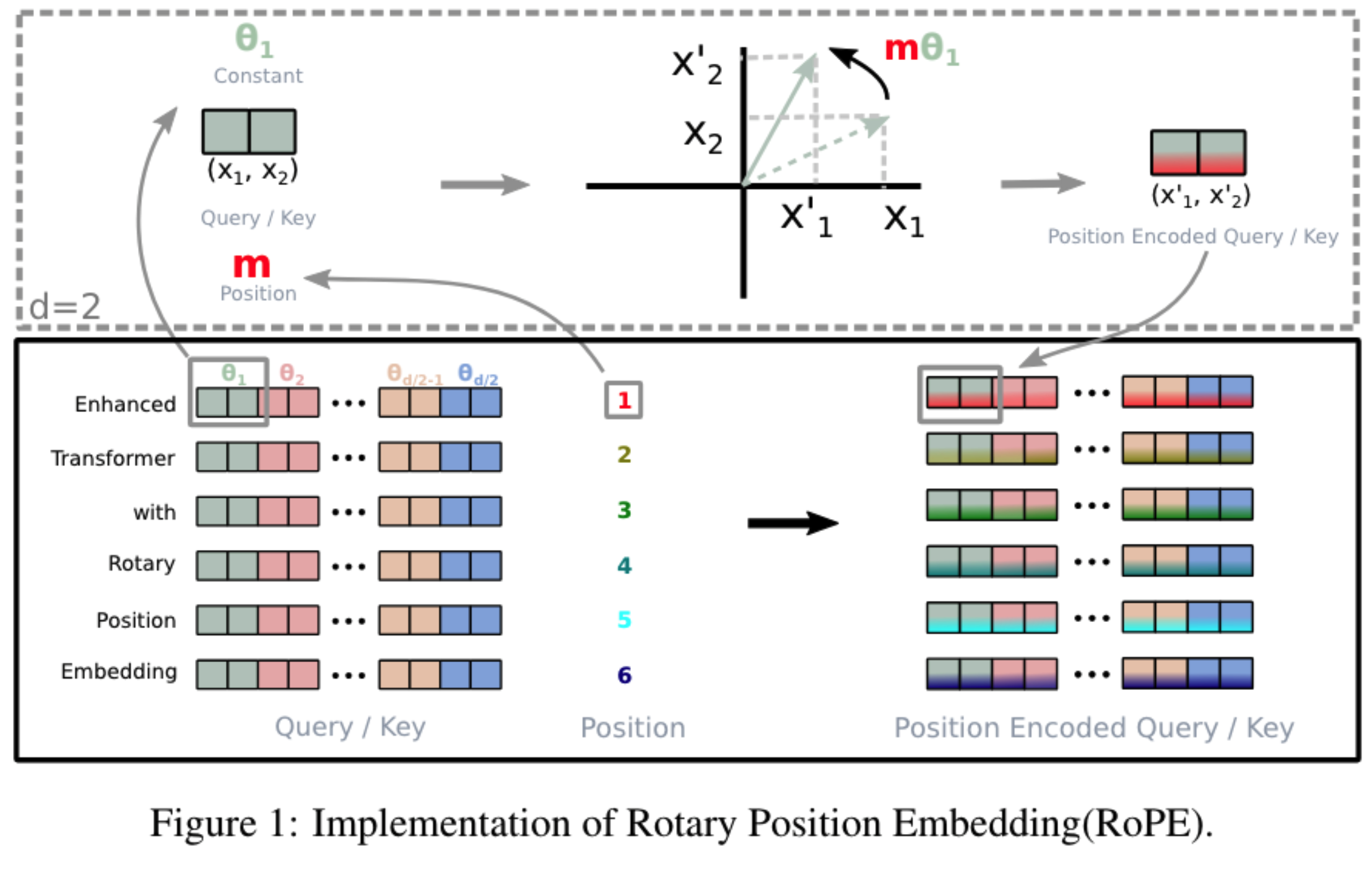
Rotary Positional Encoding is a type of position encoding that encodes absolute positional information with a rotation matrix and naturally incorporates explicit relative position dependency in self-attention formulation

we’ve generated a separate positional encoding vector and added it to our token embedding prior to our Q, K and V projections. By adding the positional information directly to our token embedding, we are polluting the semantic information with the positional information. $$ R(m\theta) = \begin{bmatrix} \cos(m\theta) & -\sin(m\theta) \ \sin(m\theta) & \cos(m\theta) \end{bmatrix} $$

The challenge with this solution was that it works only for 2D. Hence, the authors came up with a solution that takes token pairs. This is why ROPE embeddings require dimensions of even length.

KV Caching

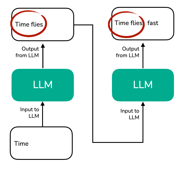
When we implement an LLM text generation function, we typically only use the last generated token from each step. However, the visualization above highlights one of the main inefficiencies on a conceptual level. This inefficiency (or redundancy) becomes more clear if we zoom in on the attention mechanism itself.

LLMs generate one word (or token) at a time. Suppose the LLM generated the word “fast” so that the prompt for the next round becomes “Time flies fast”. This is illustrated in the next figure below: As we can see, based on comparing the previous 2 figures, the keys and value vectors for the first two tokens are exactly the same, and it would be wasteful to recompute them in each next-token text generation round.

Now, the idea of the KV cache is to implement a caching mechanism that stores the previously generated key and value vectors for reuse, which helps us to avoid these unnecessary recomputations.

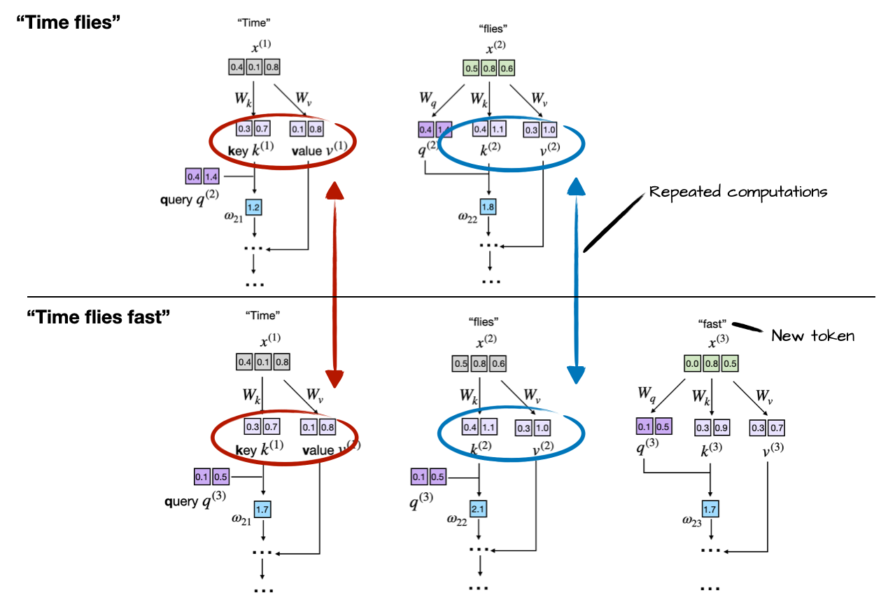
Notice the redundancy: tokens “Time” and “flies” are recomputed at every new generation step. The KV cache resolves this inefficiency by storing and reusing previously computed key and value vectors:

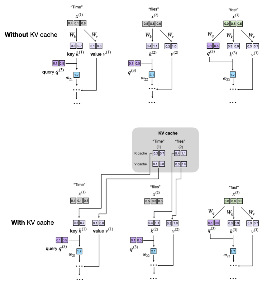
Initially, the model computes and caches key and value vectors for the input tokens.
For each new token generated, the model only computes key and value vectors for that specific token.
Previously computed vectors are retrieved from the cache to avoid redundant computations.

As sequence length increases, the benefits and downsides of a KV cache become more pronounced in the following ways:

[Good] Computational efficiency increases: Without caching, the attention at step t must compare the new query with t previous keys, so the cumulative work scales quadratically, O(n²). With a cache, each key and value is computed once and then reused, reducing the total per-step complexity to linear, O(n).
[Bad] Memory usage increases linearly: Each new token appends to the KV cache. For long sequences and larger LLMs, the cumulative KV cache grows larger, which can consume a significant or even prohibitive amount of (GPU) memory. As a workaround, we can truncate the KV cache, but this adds even more complexity (but again, it may well be worth it when deploying LLMs.)

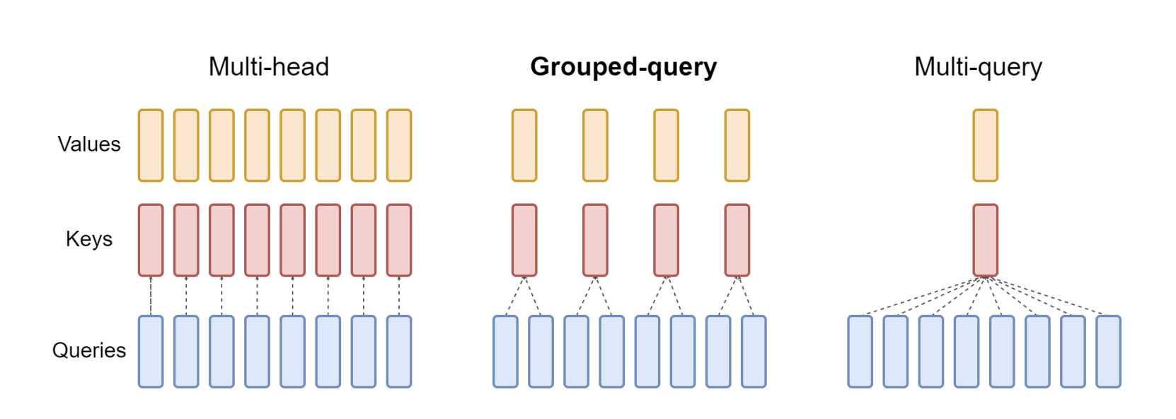
Grouped Query Attention

Grouped-query attention (GQA) is a simple approach that blends elements of multi-head attention (MHA) and multi-query attention (MQA) to create a more efficient attention mechanism. The mathematical framework of GQA can be understood as follows:

Division into Groups: In GQA, the query heads (Q) from a traditional multi-head model are divided into G groups. Each group is assigned a single key (K) and value (V) head. This configuration is denoted as GQA-G, where G represents the number of groups. We mean-pool the key and value projection matrices of the original heads within each group to convert a multi-head model into a GQA model. This technique averages the projection matrices of each head in a group, resulting in a single key and value projection for that group.

By utilizing GQA, the model maintains a balance between MHA quality and MQA speed. Because there are fewer key-value pairs, memory bandwidth and data loading needs are minimized. The choice of G presents a trade-off: more groups (closer to MHA) result in higher quality but slower performance, whereas fewer groups (near to MQA) boost speed at the risk of sacrificing quality. Furthermore, as the model size grows, GQA allows for a proportional decrease in memory bandwidth and model capacity, corresponding with the model’s scale. In contrast, for bigger models, the reduction to a single key and value head can be unduly severe in MQA.

#LLM #Notes