XGBoost eXtreme Gradient Boosting

XgBoost is used for both Regression and Classification. XGBoost (eXtreme Gradient Boosting) is an advanced implementation of gradient boosting algorithm.

When to use XGBoost?

Tabular Data: XGBoost is particularly well-suited for structured, tabular data, such as data stored in CSV files or SQL databases.
Large Datasets: XGBoost’s efficiency and parallel processing capabilities make it an excellent choice for handling large datasets with numerous features.
Feature Importance: XGBoost provides built-in feature importance scores, allowing you to identify the most influential variables in your model.
Imbalanced Data: XGBoost offers hyperparameters, such as scale_pos_weight, which can be used to address class imbalance in the data, making it effective for imbalanced classification problems.

Regression

We are given input features (X) and target feature (Y). Now we start with a default set of predictions (by default set to 0.5 in both classification and regression but you can start from other values as well)
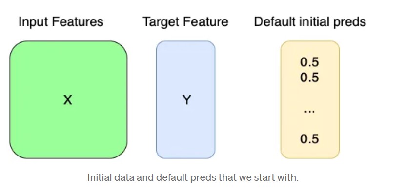
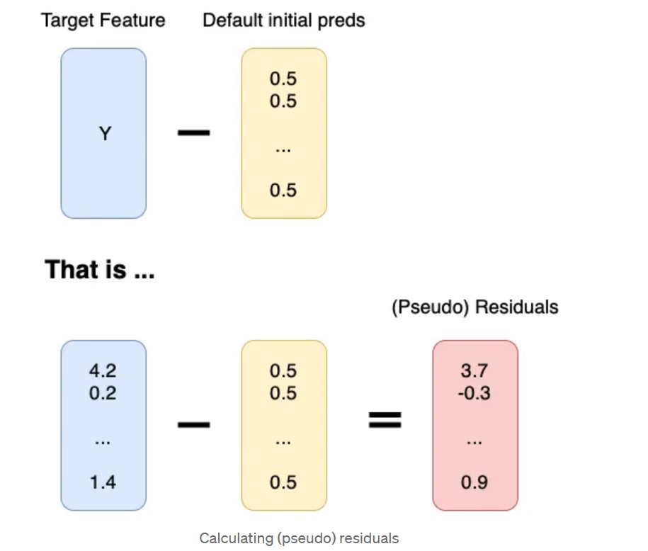
Calculate the (pseudo) residuals by subtracting Y from default initial preds.
Building XGBoost Trees Now we go through all the input features one by one.
- Select the first feature, sort it’s values in ascending order and go through those values one by one.
- Take 2 points at a time from the start, get the mean of those 2 values and then divide the leaf residuals according to the mean value, i.e. put residuals of elements with less than mean feature value to one node and the others to a different node.
- Do this for all features and all values in each feature.
- We now calculate the gain value for each of the splits created in step 3 as shown below.
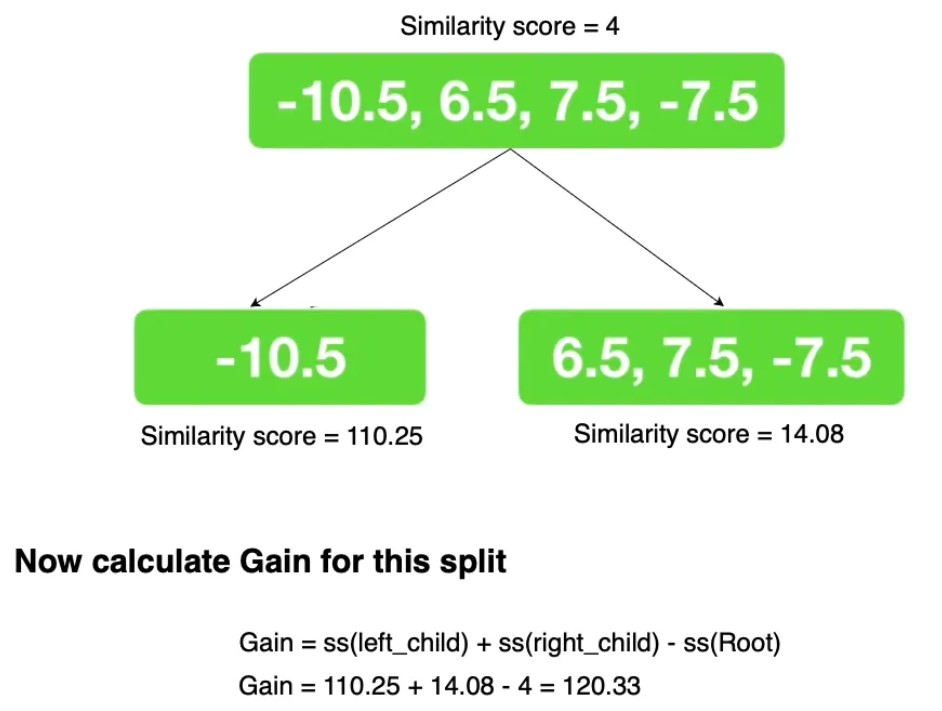
Creating the tree We continue doing step 3 & 4 for the children of the tree to split it further. The stopping conditions are either the max depth has been reached (6 by default) or the leaf has just minimum amount of residuals in it
Pruning the tree We use a hyper parameter gamma(r) to prune trees. We go bottom up from the tree while pruning. If the Gain of a parent node is less than the gamma (r) value then we prune its children (more formally if gain-r < 0). We only go up if we pruned at that particular point else we stop there.
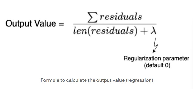
Calculating the output Value Now we’ll calculate the output values for each of the child nodes in the tree using the following formula.

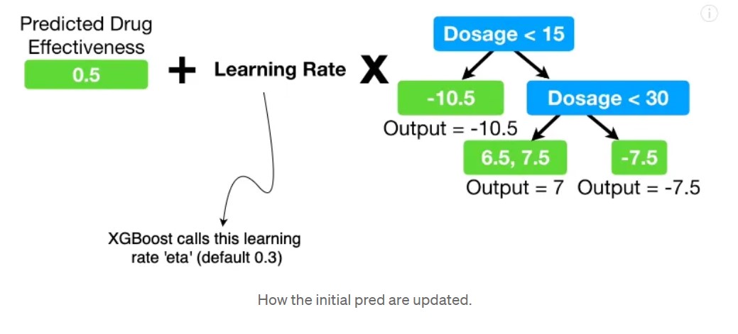
Now that we have a tree that can predict residuals, we can update are initial default vector of 0.5 predictions by adding these residuals to it (multiplied by a learning rate ofcourse. We don’t want to directly go to the pred value and overfit) GBM

Classification

Given data and initial predictions(same as above)
Calculating Pseudo Residuals(same as above)
Building XGBoost Trees
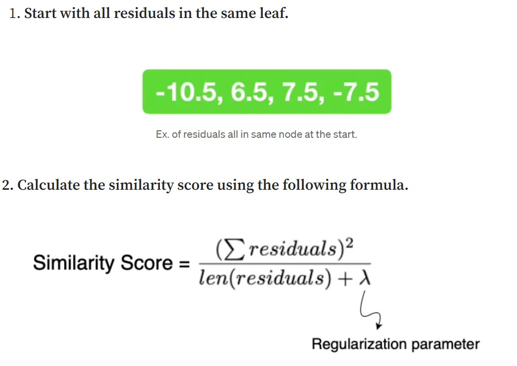
- Start with all residuals in the same leaf [ 0.5 , -0.5, 0.5 , 0.5 ]
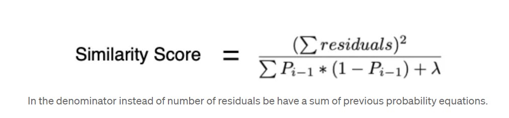
- Like we did in regression, we will calculate similarity score for nodes. Although the formula changes slightly for classification.
- Finding the best splitting feature and its values. Go through all of the features one by one. Then sort all values in a feature and go through the values one by one. Find the mean of 2 values at a time and split leaf values according to that value.
- 1. Calculating Gain The stopping conditions are either the max depth has been reached (6 by default) or the leaf has minimum number of residual in it (calculated using cover).

What is ‘cover’? Cover is basically defined as the denominator of similarity score minus lambda. So basically the formula is… GBM By default the value of cover is set to 1 in both cases. Regression: Since the minimum value of cover is 1 by default and we cant have less that 1 residuals in a leaf cover has no effect on how we grow the tree for the default value of cover. Classification: If the calculated cover value for a leaf is less than 1 then we discard that division (essentially pruning the left)

Pruning the tree Start bottom up and just prune based on the hyper-parameter gamma (r) and gain for each node.
Calculating Output Calculating the output value at each node. Heres the formula. As you can see its quite similar to what we saw in Regression.
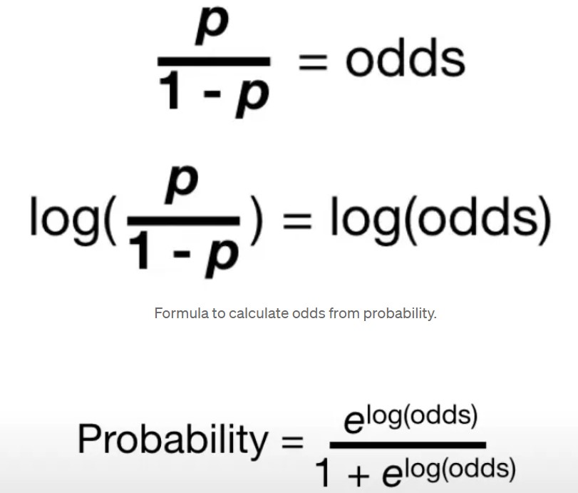
Updating the residuals and getting the output But wait this isn’t regression and we cant simply add these values (multiplied by learning rate(eta)). We need to convert the initial probability (0.5) into log(odds), perform the addition with lr multiplied and convert it back to probability. Let’s take it step by step. Okay now we have all of the tools and understanding necessary for the next step.
- Convert the default initial probability (0.5) to log(odds). So that is, log(odds) = log(p/(1-p)) = log(0.5/1–0.5) = log(0.5/0.5) = log(1) = 0
- Perform the step of adding the node value multiplied by lr Log(odds) Prediction = 0 + 0.3*(-2) = -0.6
- Convert this log(odds) value back to probability using the second formula. Probability = e^(-0.6)/1+e^(-0.6) = 0.35

Key Features of XGBoost

Regularization: XGBoost employs both L1 (LASSO) and L2 (Ridge) regularization techniques to prevent overfitting, which enhances model generalization
Parallel Processing: It supports parallel computation, allowing it to build trees efficiently by splitting nodes simultaneously
Handling Missing Data: The algorithm can automatically handle missing values during training, which simplifies preprocessing steps
Built-in Cross-Validation: XGBoost has a built-in cross-validation feature that helps in tuning hyperparameters and reduces the risk of overfitting.
Flexibility: It can be applied to various tasks including classification, regression, and ranking problems

Learning Rate (Shrinkage): This parameter controls how much each tree contributes to the final prediction. A smaller learning rate often leads to better accuracy but requires more trees Tree Pruning: Unlike traditional methods that grow trees fully before pruning, XGBoost prunes trees backward from the leaves to avoid overfitting and improve efficiency

XGBoost Alternatives: XGBoost vs CatBoost vs LightGBM

CatBoost and LightGBM are gradient boosting algorithms that share similarities with XGBoost in their ability to handle supervised learning tasks. CatBoost excels in handling categorical features without the need for preprocessing, making it user-friendly and robust to overfitting. It offers efficient training speed and memory usage, but may have limited flexibility in hyperparameter tuning compared to XGBoost. LightGBM, on the other hand, utilises a histogram-based algorithm for unparalleled speed and efficiency, particularly with large datasets and high-dimensional features. It supports parallel and GPU training, delivering fast performance, but may be prone to overfitting on smaller datasets.

When considering which algorithm to choose, XGBoost is a versatile option with extensive hyperparameter tuning capabilities, strong community support, and robustness in handling missing data and sparse inputs. CatBoost is ideal for datasets with categorical features and when computational resources are limited, while LightGBM shines in scenarios requiring fast training speeds and efficient memory usage, especially on large-scale datasets. Ultimately, the choice depends on the specific characteristics of the dataset, available computational resources, and the specific requirements of the task at hand.

The optimal algorithm to use often varies based on both the dataset nuances and your performance requirements. Don’t hesitate to experiment with all three; a less theoretically ‘perfect’ model might surprise you in practice. Also, remember that XGBoost, CatBoost, and LightGBM are constantly evolving. Updates and improvements may reshape their performance characteristics over time, making it worthwhile to revisit your algorithm choices periodically.

LightGBM

Histogram-based algorithms

Histogram-based algorithms are advanced techniques primarily used in machine learning to enhance the efficiency of training models, particularly in gradient boosting methods. They leverage the concept of histograms to optimize the decision tree construction process. Binning: Continuous feature values are divided into discrete intervals or “bins.” This transformation simplifies the data representation, making it easier to manage and compute. Histogram Construction: Each feature’s values are aggregated into histograms that represent the distribution of values across these bins. This approach allows for efficient computations and reduces the complexity of finding optimal split points during model training

How the Histogram-based Algorithm Works

Binning
- Instead of using the raw continuous values of a feature, the histogram-based algorithm discretizes these values by placing them into bins. This step reduces the number of unique values that need to be evaluated as potential split points.
- For each feature, a predefined number of bins (typically determined by a hyperparameter) is created. Each continuous feature value is assigned to one of these bins based on its range.
- This process transforms the continuous feature space into a smaller set of intervals (or bins), reducing the number of candidate splits to the number of bins.
Building Histograms for Gradient Statistics
- After binning the feature values, the algorithm creates histograms for each feature. These histograms store aggregated information, such as: The sum of the gradients of the instances falling into each bin. The sum of the Hessian values (second-order gradients) of the instances in each bin (used in second-order methods like LightGBM).
- The histogram for each feature is essentially a compact summary of how the instances are distributed across the bins and how their gradient values are distributed.
Finding the Optimal Split:
- Once the histograms are built, the algorithm evaluates the potential split points. Instead of evaluating all possible continuous values, it evaluates the split points corresponding to the boundaries between adjacent bins.
- For each possible split point (i.e., bin boundary), the algorithm calculates the information gain or loss reduction by splitting the histogram at that boundary.
- The split that maximizes the information gain is selected as the optimal split point for that feature.
Histogram Subtraction (Speeding Up Subsequent Splits):
- A key optimization in the histogram-based algorithm is histogram subtraction. When a node is split, the histograms for the child nodes can be computed efficiently by subtracting the histograms of the left and right children from the parent node’s histogram. This avoids recalculating histograms from scratch for every split, speeding up the process

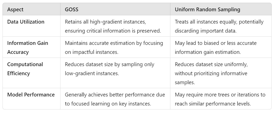
Gradient-based One-Side Sampling

Traditional sampling methods, such as uniform random sampling, may either discard valuable information or retain too much redundant data, leading to inefficiencies or suboptimal model performance.

GOSS is a sampling technique that selectively retains data instances based on the magnitude of their gradients (i.e., the first-order derivatives of the loss function with respect to the predictions). In the context of GBDT:

Gradients indicate the direction and magnitude by which the model should adjust to minimize the loss.
Large gradients correspond to instances where the model is underperforming, signaling areas that require more attention.
Small gradients suggest that the model is performing adequately on those instances. GOSS leverages this gradient information to retain all instances with large gradients (ensuring that the model focuses on areas needing improvement) and randomly samples from instances with small gradients (maintaining computational efficiency by reducing the dataset size without significant loss of information).

Thought for 4 seconds

Gradient-based One-Side Sampling (GOSS) in LightGBM

Gradient-based One-Side Sampling (GOSS) is a key optimization technique employed by LightGBM, a highly efficient gradient boosting framework. GOSS enhances the training speed and scalability of Gradient Boosted Decision Trees (GBDT) without compromising model accuracy. This method intelligently selects data instances for constructing decision trees based on their gradient information, ensuring that the most informative samples are prioritized during training.

Overview of LightGBM and Its Training Challenges LightGBM is renowned for its speed and efficiency in handling large-scale datasets. It achieves this through several innovative strategies, including:

Histogram-based algorithms for faster split finding. Leaf-wise tree growth for deeper and more accurate trees. GOSS for effective data sampling. Despite these optimizations, training GBDT models on massive datasets remains computationally intensive. Traditional sampling methods, such as uniform random sampling, may either discard valuable information or retain too much redundant data, leading to inefficiencies or suboptimal model performance.

What is Gradient-based One-Side Sampling (GOSS)? GOSS is a sampling technique that selectively retains data instances based on the magnitude of their gradients (i.e., the first-order derivatives of the loss function with respect to the predictions). In the context of GBDT:

Gradients indicate the direction and magnitude by which the model should adjust to minimize the loss. Large gradients correspond to instances where the model is underperforming, signaling areas that require more attention. Small gradients suggest that the model is performing adequately on those instances. GOSS leverages this gradient information to retain all instances with large gradients (ensuring that the model focuses on areas needing improvement) and randomly samples from instances with small gradients (maintaining computational efficiency by reducing the dataset size without significant loss of information).

How GOSS Works in LightGBM?

Compute Gradients and Hessians:
- For each data instance, LightGBM calculates the gradient (first-order derivative) and Hessian (second-order derivative) based on the current model’s predictions and the chosen loss function.
Rank Instances by Gradient Magnitude:
- Instances are sorted in descending order based on the absolute value of their gradients. Those with larger gradients are more critical for model improvement.
Select Instances to Retain and Sample:
- Retain All High-Gradient Instances: A predefined proportion (e.g., the top 20%) of instances with the largest gradients is retained in their entirety. These instances are deemed highly informative for identifying optimal split points.
- Sample from Low-Gradient Instances The remaining instances (e.g., the bottom 80%) with smaller gradients are randomly sampled at a lower rate (e.g., 20% of these instances). This reduces the overall number of data points without significantly impacting the model’s ability to generalize.
Reweight Sampled Instances: To maintain an unbiased estimate of the information gain, the sampled low-gradient instances are assigned a weight inversely proportional to their sampling rate. This ensures that their reduced presence in the dataset does not skew the model’s learning process.
Construct Histograms and Build Trees: Using the retained and sampled instances, LightGBM constructs histograms for each feature to identify optimal split points efficiently. The trees are grown based on these histograms, focusing on the most informative splits derived from the high-gradient instances.

GBM LightGBM’s leaf-wise approach grows trees by splitting the leaf with the maximum potential to reduce loss, rather than level-wise. GOSS ensures that the data used to evaluate these splits is both informative and efficiently sampled.

Exclusive Feature Bundling (EFB)

Exclusive Feature Bundling (EFB) is a powerful optimization technique employed by LightGBM, a popular Gradient Boosted Decision Tree (GBDT) framework. EFB is specifically designed to handle high-dimensional and sparse datasets efficiently by reducing the number of features without significant loss of information. This optimization leads to lower memory consumption and faster computation, enabling LightGBM to scale effectively to large datasets.

High-Dimensional Data: Datasets with a vast number of features (columns), common in domains like text processing (e.g., one-hot encoded text), genomics, and recommendation systems. Sparsity: Many features contain a large number of zero or missing values. For example, in one-hot encoding, only one feature per category is active (non-zero) for each instance, while the rest are zero. Memory Consumption: Storing and processing numerous sparse features can be memory-intensive. Computational Efficiency: Evaluating splits across many features increases computational time, especially when many features are rarely active. Exclusive Feature Bundling is an algorithmic strategy that aggregates mutually exclusive features—features that are unlikely to be non-zero simultaneously—into a single composite feature. By doing so, EFB effectively reduces the feature space dimensionality without losing critical information required for model training.

How Exclusive Feature Bundling Works

Analyze Feature Activity:
Determine Exclusivity:
- Two features are considered mutually exclusive if there is no instance where both features are active simultaneously.
- Formally, for features fi and fj are mutually exclusive if for all x, x belongs to Data , fi(x) X fj(x) = 0
Group features into bundles where within each bundle, features are pairwise mutually exclusive

Steps in Merging Features Using EFB

Identifying Exclusive Features The first step involves identifying features that are mutually exclusive, meaning they do not take non-zero values simultaneously. This is crucial in high-dimensional data where many features may be sparsely populated.
Conflict Graph Construction A conflict graph is created where:
- Each feature is represented as a vertex.
- An edge is drawn between two vertices if the corresponding features can take non-zero values at the same time. The goal is to minimize conflicts by bundling features that do not conflict with each other.
Greedy Bundling Algorithm LightGBM employs a Greedy Bundling Algorithm to determine which features can be bundled together: The algorithm sorts the features based on their degree (the number of edges connected to them). It iteratively checks each feature against existing bundles to see if it can be added without exceeding a predefined conflict count (K). If a feature cannot be added to any existing bundle due to conflicts, it is placed in a new bundle.
Merging Exclusive Features Once bundles are formed, the next step is to merge these features: For each bundle, LightGBM creates a new feature that combines the values of all exclusive features in that bundle. The merging process involves creating a new histogram for the bundled feature, which aggregates the bin counts from individual features.
Histogram Construction During histogram construction for the merged features, LightGBM calculates bin ranges and assigns values based on the presence of non-zero entries from the original features. This reduces the complexity of histogram building from O(data× features) to O( data× bundles), where the number of bundles is significantly less than the number of original features.
Output of Bundled Features The final output consists of fewer features (bundles) that retain the essential information needed for model training while simplifying computations.

Catboost

One main difference between CatBoost and other boosting algorithms is that the CatBoost implements symmetric trees. This may sound crazy but helps in decreasing prediction time, which is extremely important for low latency environments.

Symmetric Trees

Symmetric Trees are a type of decision tree where each level of the tree is structured identically, meaning that all nodes at a particular depth share the same split condition. This contrasts with traditional asymmetric trees, where each node can have its own unique split condition, leading to an irregular and unbalanced tree structure.

In Asymmetric Trees:

Each node independently selects the best feature and threshold to split the data
Leads to trees where different branches can have varying depths and structures.
Flexibility: Can capture complex patterns and interactions within the data.
Higher Accuracy: Potentially better performance on diverse datasets due to their adaptability.
Computationally Intensive: More split conditions to evaluate, leading to longer training times.
Memory Consumption: Requires more memory to store varied split conditions.
Prediction Speed: Traversing an irregular tree can be slower, especially for deep trees. In Symmetric Trees
All nodes at the same depth share the same split condition (feature and threshold).
Results in a balanced and uniform tree structure.
Computational Efficiency: Fewer split conditions to evaluate, reducing training time.
Memory Optimization: Shared split conditions lower memory usage.
Faster Predictions: Uniform structure allows for optimized traversal algorithms, speeding up inference.
Reduced Flexibility: May not capture intricate patterns as effectively as asymmetric trees.
Potentially Lower Accuracy: The enforced uniformity can sometimes lead to suboptimal splits for certain nodes.

How CatBoost Implements Symmetric Trees

Initialization:
- Start with an initial prediction (e.g., the mean of the target variable).
Iterative Boosting: -For each boosting iteration: Compute gradients and Hessians based on the current loss function. Construct a new symmetric tree to model these gradients.
Symmetric Split Determination: At each depth level:
- Feature Selection: Choose the best feature and threshold that maximizes information gain or minimizes the loss.
- Uniform Application: Apply the selected split condition uniformly across all nodes at that depth.
Leaf Value Calculation:
- Compute the output value for each leaf based on the aggregated gradients and Hessians.
Model Update:
- Update the model’s predictions by adding the contributions from the new tree, scaled by the learning rate.

Categorical Features

Traditional Approaches to Handling Categorical Features Before diving into CatBoost’s methodologies, it’s beneficial to understand conventional techniques: a. One-Hot Encoding Method: Creates binary columns for each category within a feature. Pros: Simple and effective for nominal data without intrinsic order. Cons: High Dimensionality: Can lead to a significant increase in feature space, especially with high cardinality. Sparse Data: Results in many zero entries, which can be memory inefficient. b. Label Encoding Method: Assigns a unique integer to each category. Pros: Simple and maintains the original feature’s dimensionality. Cons: Implicit Ordinality: Introduces an unintended ordinal relationship, potentially misleading models that interpret higher integers as more significant. c. Target Encoding (Mean Encoding) Method: Replaces categories with a statistic (e.g., mean target value) calculated from the training data. Pros: Captures the relationship between categories and the target variable. Cons: Overfitting Risk: Categories with few samples can lead to noisy estimates. Target Leakage: Without proper handling, the encoding can leak information from the target into the features.

Ordered Target Statistics

Definition: A technique where categorical features are encoded based on statistics derived from the target variable, computed in a manner that prevents target leakage. CatBoost permutes the dataset to ensure randomness and reduce bias. For each instance in the permuted data:

Compute Statistics: Calculate the mean target value for the category using only the data points that precede the current instance in the permutation.
Assign Encoded Value: Replace the categorical feature with the computed statistic.
Averaging: Smooth the encoded values by combining them with global statistics (e.g., overall mean) to handle categories with few instances. Consider a binary classification problem with a categorical feature “Color”:

Instance Color Target 1 Red 0 2 Blue 1 3 Green 0 4 Red 1 5 Blue 0 Assuming a permutation order: [3, 1, 4, 2, 5]

Instance 3 (Green): No preceding data. Encoded as global mean, say 0.4. Instance 1 (Red): No preceding “Red”. Encoded as global mean, 0.4. Instance 4 (Red): One preceding “Red” with target 0. Encoded as 0. Instance 2 (Blue): No preceding “Blue”. Encoded as global mean, 0.4. Instance 5 (Blue): One preceding “Blue” with target 1. Encoded as 1. Resulting Encoded Feature:

Instance Encoded Color 3 0.4 1 0.4 4 0 2 0.4 5 1

Permutation-Driven Encoding

An extension of ordered target statistics where multiple permutations are used to stabilize the encoding and reduce variance. Multiple Permutations: CatBoost generates several random permutations of the dataset. Aggregate Statistics: For each permutation, compute ordered target statistics as described above. Average Encoded Values: Combine the encodings from all permutations to obtain a final, robust encoded value for each categorical feature. Advantages: Stabilizes Encodings: Reduces the variance introduced by a single permutation, leading to more reliable encodings. Enhances Generalization: Mitigates the risk of overfitting by averaging across multiple views of the data.

Bayesian Averaging

A smoothing technique applied to target statistics to handle categories with few instances, preventing overfitting and extreme values.

Global Statistics: Compute the global mean of the target variable across all data.
Category Statistics: For each category, compute the mean target value based on ordered target statistics.
Apply Smoothing: Combine category-specific statistics with the global mean using a predefined smoothing factor, especially for categories with limited data. Encoded Value= (n⋅Category Mean+k⋅Global Mean)/(n+k) n = Number of instances in the category. k = Smoothing parameter (controls the weight given to the global mean).

Leaf Values

In the context of decision trees, a leaf is a terminal node that provides the final output for instances that traverse the tree following specific decision paths. The leaf value is the prediction assigned to any instance that lands in that particular leaf during inference. CatBoost calculates gradients and Hessians (second-order derivatives) of the loss function to determine optimal leaf values.

Leaf Value = - sum(gradient)/(sum(hessian)+lambda)

2. Sample Dataset

Consider a simple binary classification dataset:

Instance	Feature A	Feature B	Category (Color)	Target
1	2.5	3.1	Red	0
2	1.3	2.2	Blue	1
3	3.3	1.8	Green	0
4	2.1	4.0	Red	1
5	1.8	3.5	Blue	0
6	3.0	2.9	Green	1
7	2.7	3.3	Red	0
8	1.5	2.7	Blue	1
9	3.1	1.9	Green	0
10	2.4	3.6	Red	1

3. Initial Prediction

Before any trees are built, CatBoost initializes the model’s predictions. Typically, this is the global mean of the target variable.

[ \text{Initial Prediction} (\hat{y}^{(0)}) = \frac{\sum \text{Target}}{\text{Number of Instances}} = \frac{5}{10} = 0.5 ]

4. First Iteration: Building the First Tree

a. Compute Residuals

[ \text{Residual}_i^{(1)} = \text{Target}_i - \hat{y}^{(0)} = \text{Target}_i - 0.5 ]

Instance	Residual
1	-0.5
2	0.5
3	-0.5
4	0.5
5	-0.5
6	0.5
7	-0.5
8	0.5
9	-0.5
10	0.5

b. Calculate Gradients and Hessians

Assuming a squared error loss:

[ g_i = -2 \times \text{Residual}_i = -2r_i ] [ h_i = 2 ]

Instance	Gradient (( g_i ))	Hessian (( h_i ))
1	1.0	2
2	-1.0	2
3	1.0	2
4	-1.0	2
5	1.0	2
6	-1.0	2
7	1.0	2
8	-1.0	2
9	1.0	2
10	-1.0	2

c. Build a Symmetric Tree

Split Condition: Suppose the best split is on Feature A ≤ 2.0.

Depth 0: Feature A ≤ 2.0
├── Left Leaf: Feature A ≤ 2.0
└── Right Leaf: Feature A > 2.0

d. Assign Residuals to Leaves

Left Leaf: Instances where Feature A ≤ 2.0 → Instances 2, 5, 8
Right Leaf: Instances where Feature A > 2.0 → Instances 1, 3, 4, 6, 7, 9, 10

e. Compute Leaf Values

[ \text{Leaf Value} = -\frac{\sum g_i}{\sum h_i + \lambda} ]

Assume Regularization Parameter (( \lambda )) = 1

Left Leaf: [ \text{Leaf Value} = -\frac{(-1.0) + (1.0) + (-1.0)}{(2 + 2 + 2) + 1} = -\frac{-1.0}{7} \approx 0.143 ]
Right Leaf: [ \text{Leaf Value} = -\frac{(1.0) + (1.0) + (-1.0) + (1.0) + (1.0) + (1.0) + (1.0)}{(2 + 2 + 2 + 2 + 2 + 2 + 2) + 1} = -\frac{5.0}{15} \approx -0.333 ]

f. Update Predictions

[ \hat{y}_i^{(1)} = \hat{y}_i^{(0)} + \eta \times \text{Leaf Value} ]

Assume Learning Rate (( \eta )) = 1 for simplicity.

Instance	Leaf Assignment	Leaf Value	Updated Prediction (( \hat{y}^{(1)} ))
1	Right	-0.333	0.5 - 0.333 = 0.167
2	Left	0.143	0.5 + 0.143 = 0.643
3	Right	-0.333	0.5 - 0.333 = 0.167
4	Right	-0.333	0.5 - 0.333 = 0.167
5	Left	0.143	0.5 + 0.143 = 0.643
6	Right	-0.333	0.5 - 0.333 = 0.167
7	Right	-0.333	0.5 - 0.333 = 0.167
8	Left	0.143	0.5 + 0.143 = 0.643
9	Right	-0.333	0.5 - 0.333 = 0.167
10	Right	-0.333	0.5 - 0.333 = 0.167

5. Second Iteration: Building the Second Tree

a. Compute New Residuals

[ \text{Residual}_i^{(2)} = \text{Target}_i - \hat{y}_i^{(1)} ]

Instance	Target	Updated Prediction (( \hat{y}^{(1)} ))	Residual
1	0	0.167	-0.167
2	1	0.643	0.357
3	0	0.167	-0.167
4	1	0.167	0.833
5	0	0.643	-0.643
6	1	0.167	0.833
7	0	0.167	-0.167
8	1	0.643	0.357
9	0	0.167	-0.167
10	1	0.167	0.833

b. Calculate Gradients and Hessians

[ g_i = -2 \times \text{Residual}_i ] [ h_i = 2 ]

Instance	Residual	Gradient (( g_i ))	Hessian (( h_i ))
1	-0.167	0.333	2
2	0.357	-0.714	2
3	-0.167	0.333	2
4	0.833	-1.666	2
5	-0.643	1.286	2
6	0.833	-1.666	2
7	-0.167	0.333	2
8	0.357	-0.714	2
9	-0.167	0.333	2
10	0.833	-1.666	2

c. Build the Second Symmetric Tree

Split Condition: Suppose the best split is on Feature B ≤ 3.0.

Depth 0: Feature B ≤ 3.0
├── Left Leaf: Feature B ≤ 3.0
└── Right Leaf: Feature B > 3.0

d. Assign Residuals to Leaves

Left Leaf: Instances where Feature B ≤ 3.0 → Instances 1, 2, 3, 7, 8, 9, 10
Right Leaf: Instances where Feature B > 3.0 → Instances 4, 5, 6

e. Compute Leaf Values

[ \text{Leaf Value} = -\frac{\sum g_i}{\sum h_i + \lambda} ]

Left Leaf: [ \text{Leaf Value} = -\frac{0.333 + (-0.714) + 0.333 + 0.333 + (-0.714) + 0.333 + (-1.666)}{(2 \times 7) + 1} = -\frac{-1.642}{15} \approx 0.109 ]
Right Leaf: [ \text{Leaf Value} = -\frac{(-1.666) + 1.286 + (-1.666)}{(2 \times 3) + 1} = -\frac{-1.046}{7} \approx 0.149 ]

f. Update Predictions

[ \hat{y}_i^{(2)} = \hat{y}_i^{(1)} + \eta \times \text{Leaf Value} ]

Assume Learning Rate (( \eta )) = 1 for simplicity.

Instance	Leaf Assignment	Leaf Value	Updated Prediction (( \hat{y}^{(2)} ))
1	Left	0.109	0.167 + 0.109 = 0.276
2	Left	0.109	0.643 + 0.109 = 0.752
3	Left	0.109	0.167 + 0.109 = 0.276
4	Right	0.149	0.167 + 0.149 = 0.316
5	Right	0.149	0.643 + 0.149 = 0.792
6	Right	0.149	0.167 + 0.149 = 0.316
7	Left	0.109	0.167 + 0.109 = 0.276
8	Left	0.109	0.643 + 0.109 = 0.752
9	Left	0.109	0.167 + 0.109 = 0.276
10	Left	0.109	0.167 + 0.109 = 0.276

6. Visualization of Leaf Value Assignment

Below is a graphical representation of the two iterations, showcasing how leaf values are assigned and predictions are updated.

a. First Iteration

Symmetric Tree (Iteration 1)

          Feature A ≤ 2.0
           /          \
   Leaf Value: 0.143   Leaf Value: -0.333
        /                    \
Instances 2,5,8           Instances 1,3,4,6,7,9,10

Prediction Update:
- Instances 2,5,8: 0.5 + 0.143 = 0.643
- Instances 1,3,4,6,7,9,10: 0.5 - 0.333 = 0.167

b. Second Iteration

Symmetric Tree (Iteration 2)

          Feature B ≤ 3.0
           /          \
   Leaf Value: 0.109   Leaf Value: 0.149
        /                    \
Instances 1,2,3,7,8,9,10   Instances 4,5,6

Prediction Update:
- Instances 1,2,3,7,8,9,10: Previous Prediction + 0.109
- Instances 4,5,6: Previous Prediction + 0.149

c. Summary Table

Iteration	Instance	Leaf Assignment	Leaf Value	Updated Prediction
0	All	N/A	N/A	0.5
1	2,5,8	Left	0.143	0.643
1	1,3,4,6,7,9,10	Right	-0.333	0.167
2	1,2,3,7,8,9,10	Left	0.109	0.276 (for 1,3,7,9,10), 0.752 (for 2,8)
2	4,5,6	Right	0.149	0.316 (for 4,6), 0.792 (for 5)

7. Key Insights

Symmetric Trees Enhance Efficiency: By applying the same split condition across all nodes at a particular depth, CatBoost reduces computational overhead and speeds up both training and inference.
Leaf Values Represent Corrections: Each leaf value adjusts the model’s predictions based on the residuals, steering the ensemble towards minimizing the loss function.
Regularization Prevents Overfitting: Parameters like ( \lambda ) and ( \eta ) control the magnitude of leaf values, ensuring that the model remains generalizable and doesn’t overfit to the training data.
Iterative Refinement: With each boosting iteration, CatBoost builds trees that progressively correct the ensemble’s errors, refining the predictions step by step.